Demo example: Using a Dataset#
This is an introduction to get started with the MetObs toolkit. These examples are making use of the demo data files that comes with the toolkit. Once the MetObs toolkit package is installed, you can import its functionality by:
[1]:
import metobs_toolkit
The Dataset#
A dataset is a collection of all observational data. Most of the methods are applied directly to a dataset. Start by creating an empty Dataset object:
[2]:
your_dataset = metobs_toolkit.Dataset()
The most relevant attributes of a Dataset are: * .df –> a pandas DataFrame where all the observational data are stored * .metadf –> a pandas DataFrame where all the metadata for each station are stored * .settings –> a Settings object to store all specific settings. * .missing_obs and .gaps –> here the missing records and gaps are stored if present.
Note that each Dataset will be equipped with the default settings.
We created a dataset and stored in under the variable ‘your_dataset’. The show method prints out an overview of data in the dataset:
[3]:
your_dataset.show() # or .get_info()
 --------  General ---------

Empty instance of a Dataset.

 --------  Settings ---------

(to show all settings use the .show_settings() method, or set show_all_settings = True)

 --------  Outliers ---------

No outliers.

 --------  Meta data ---------

No metadata is found.
TIP: to get an extensive overview of an object, call the .show() method on it.
Importing data#
To import your data into a Dataset, the following files are required:
data file: This is the CSV file containing the observations
(optional) metadata file: The CSV file containing metadata for all stations.
template file: This is a CSV file that is used to interpret your data, and metadata file (if present).
In practice, you need to start by creating a template file for your data. More information on the creation of the template can be found in the documentation (under Mapping to the toolkit).
TIP: Use the template assistant of the toolkit for creating a template file by uncommenting and running the following cell.
[4]:
# metobs_toolkit.build_template_prompt()
To import data, you must specify the paths to your data, metadata and template. For this example, we use the demo data, metadata and template that come with the toolkit.
[5]:
your_dataset.update_settings(
    input_data_file=metobs_toolkit.demo_datafile, # path to the data file
    input_metadata_file=metobs_toolkit.demo_metadatafile,
    template_file=metobs_toolkit.demo_template,
)
The settings of your Dataset are updated with the required paths. Now the data can be imported into your empty Dataset:
[6]:
your_dataset.import_data_from_file()
Inspecting the Data#
To get an overview of the data stored in your Dataset you can use
[7]:
your_dataset.show()
 --------  General ---------

Dataset instance containing:
     *28 stations
     *['temp', 'radiation_temp', 'humidity', 'precip', 'precip_sum', 'wind_speed', 'wind_gust', 'wind_direction', 'pressure', 'pressure_at_sea_level'] observation types
     *120957 observation records
     *256 records labeled as outliers
     *0 gaps
     *3 missing observations
     *records range: 2022-09-01 00:00:00+00:00 --> 2022-09-15 23:55:00+00:00 (total duration:  14 days 23:55:00)
     *time zone of the records: UTC
     *Coordinates are available for all stations.


 --------  Settings ---------

(to show all settings use the .show_settings() method, or set show_all_settings = True)

 --------  Outliers ---------

A total of 256 found with these occurrences:

{'invalid input': 256}

 --------  Meta data ---------

The following metadata is found: ['network', 'lat', 'lon', 'call_name', 'location', 'geometry', 'assumed_import_frequency', 'dataset_resolution']

 The first rows of the metadf looks like:
           network        lat       lon       call_name  location  \
name
vlinder01  Vlinder  50.980438  3.815763      Proefhoeve     Melle
vlinder02  Vlinder  51.022379  3.709695          Sterre      Gent
vlinder03  Vlinder  51.324583  4.952109         Centrum  Turnhout
vlinder04  Vlinder  51.335522  4.934732  Stadsboerderij  Turnhout
vlinder05  Vlinder  51.052655  3.675183  Watersportbaan      Gent

                           geometry assumed_import_frequency  \
name
vlinder01  POINT (3.81576 50.98044)          0 days 00:05:00
vlinder02  POINT (3.70969 51.02238)          0 days 00:05:00
vlinder03  POINT (4.95211 51.32458)          0 days 00:05:00
vlinder04  POINT (4.93473 51.33552)          0 days 00:05:00
vlinder05  POINT (3.67518 51.05266)          0 days 00:05:00

          dataset_resolution
name
vlinder01    0 days 00:05:00
vlinder02    0 days 00:05:00
vlinder03    0 days 00:05:00
vlinder04    0 days 00:05:00
vlinder05    0 days 00:05:00

 -------- Missing observations info --------

(Note: missing observations are defined on the frequency estimation of the native dataset.)
  * 3 missing observations

 name
vlinder02   2022-09-10 17:10:00+00:00
vlinder02   2022-09-10 17:15:00+00:00
vlinder02   2022-09-10 17:45:00+00:00
Name: datetime, dtype: datetime64[ns, UTC]

  * For these stations: ['vlinder02']
  * The missing observations are not filled.
(More details on the missing observation can be found in the .series and .fill_df attributes.)
None

 --------  Gaps ---------

There are no gaps.
None
If you want to inspect the data in your Dataset directly, you can take a look at the .df and .metadf attributes
[8]:
print(your_dataset.df.head())
# equivalent for the metadata
print(your_dataset.metadf.head())
                                     temp  radiation_temp  humidity  precip  \
name      datetime
vlinder01 2022-09-01 00:00:00+00:00  18.8             NaN        65     0.0
          2022-09-01 00:05:00+00:00  18.8             NaN        65     0.0
          2022-09-01 00:10:00+00:00  18.8             NaN        65     0.0
          2022-09-01 00:15:00+00:00  18.7             NaN        65     0.0
          2022-09-01 00:20:00+00:00  18.7             NaN        65     0.0

                                     precip_sum  wind_speed  wind_gust  \
name      datetime
vlinder01 2022-09-01 00:00:00+00:00         0.0         5.6       11.3
          2022-09-01 00:05:00+00:00         0.0         5.5       12.9
          2022-09-01 00:10:00+00:00         0.0         5.1       11.3
          2022-09-01 00:15:00+00:00         0.0         6.0       12.9
          2022-09-01 00:20:00+00:00         0.0         5.0       11.3

                                     wind_direction  pressure  \
name      datetime
vlinder01 2022-09-01 00:00:00+00:00              65    101739
          2022-09-01 00:05:00+00:00              75    101731
          2022-09-01 00:10:00+00:00              75    101736
          2022-09-01 00:15:00+00:00              85    101736
          2022-09-01 00:20:00+00:00              65    101733

                                     pressure_at_sea_level
name      datetime
vlinder01 2022-09-01 00:00:00+00:00               102005.0
          2022-09-01 00:05:00+00:00               101997.0
          2022-09-01 00:10:00+00:00               102002.0
          2022-09-01 00:15:00+00:00               102002.0
          2022-09-01 00:20:00+00:00               101999.0
           network        lat       lon       call_name  location  \
name
vlinder01  Vlinder  50.980438  3.815763      Proefhoeve     Melle
vlinder02  Vlinder  51.022379  3.709695          Sterre      Gent
vlinder03  Vlinder  51.324583  4.952109         Centrum  Turnhout
vlinder04  Vlinder  51.335522  4.934732  Stadsboerderij  Turnhout
vlinder05  Vlinder  51.052655  3.675183  Watersportbaan      Gent

                           geometry  lcz assumed_import_frequency  \
name
vlinder01  POINT (3.81576 50.98044)  NaN          0 days 00:05:00
vlinder02  POINT (3.70969 51.02238)  NaN          0 days 00:05:00
vlinder03  POINT (4.95211 51.32458)  NaN          0 days 00:05:00
vlinder04  POINT (4.93473 51.33552)  NaN          0 days 00:05:00
vlinder05  POINT (3.67518 51.05266)  NaN          0 days 00:05:00

          dataset_resolution
name
vlinder01    0 days 00:05:00
vlinder02    0 days 00:05:00
vlinder03    0 days 00:05:00
vlinder04    0 days 00:05:00
vlinder05    0 days 00:05:00
Inspecting a Station#
If you are interested in one station, you can extract all the info for that one station from the dataset by:
[9]:
favorite_station = your_dataset.get_station(stationname="vlinder02")
Favorite station now contains all the information of that one station. All methods that are applicable to a Dataset are also applicable to a Station. So to inspect your favorite station, you can:
[10]:
print(favorite_station.show())
 --------  General ---------

Dataset instance containing:
     *1 stations
     *['temp', 'radiation_temp', 'humidity', 'precip', 'precip_sum', 'wind_speed', 'wind_gust', 'wind_direction', 'pressure', 'pressure_at_sea_level'] observation types
     *4317 observation records
     *256 records labeled as outliers
     *0 gaps
     *3 missing observations
     *records range: 2022-09-01 00:00:00+00:00 --> 2022-09-15 23:55:00+00:00 (total duration:  14 days 23:55:00)
     *time zone of the records: UTC
     *Coordinates are available for all stations.


 --------  Settings ---------

(to show all settings use the .show_settings() method, or set show_all_settings = True)

 --------  Outliers ---------

A total of 256 found with these occurrences:

{'invalid input': 256}

 --------  Meta data ---------

The following metadata is found: ['network', 'lat', 'lon', 'call_name', 'location', 'geometry', 'assumed_import_frequency', 'dataset_resolution']

 The first rows of the metadf looks like:
           network        lat       lon call_name location  \
name
vlinder02  Vlinder  51.022379  3.709695    Sterre     Gent

                             geometry assumed_import_frequency  \
name
vlinder02  POINT (3.709695 51.022379)          0 days 00:05:00

          dataset_resolution
name
vlinder02    0 days 00:05:00

 -------- Missing observations info --------

(Note: missing observations are defined on the frequency estimation of the native dataset.)
  * 3 missing observations

 name
vlinder02   2022-09-10 17:10:00+00:00
vlinder02   2022-09-10 17:15:00+00:00
vlinder02   2022-09-10 17:45:00+00:00
Name: datetime, dtype: datetime64[ns, UTC]

  * For these stations: ['vlinder02']
  * The missing observations are not filled.
(More details on the missing observation can be found in the .series and .fill_df attributes.)
None

 --------  Gaps ---------

There are no gaps.
None
None
Making timeseries plots#
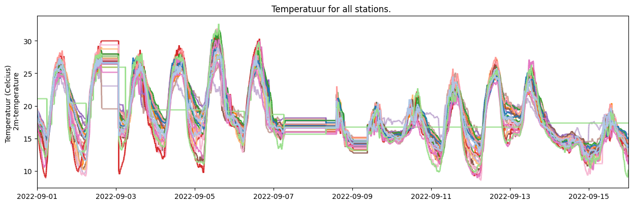
To make timeseries plots, use the following syntax to plot the temperature observations of the full Dataset:
[11]:
your_dataset.make_plot(obstype='temp')
[11]:
<Axes: title={'center': 'Temperatuur for all stations. '}, ylabel='Temperatuur (Celcius) \n 2m-temperature'>
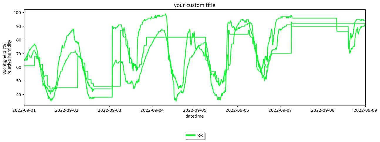
See the documentation of the make_plot() method for more details. Here an example of common used arguments.
[12]:
#Import the standard datetime library to make timestamps from datetime objects
from datetime import datetime

your_dataset.make_plot(
    # specify the names of the stations in a list, or use None to plot all of them.
    stationnames=['vlinder01', 'vlinder03', 'vlinder05'],
    # what obstype to plot (default is 'temp')
    obstype="humidity",
    # choose how to color the timeseries:
    #'name' : a specific color per station
    #'label': a specific color per quality control label
    colorby="label",
    # choose a start and endtime for the series (datetime).
    # Default is None, which uses all available data
    starttime=None,
    endtime=datetime(2022, 9, 9),
    # Specify a title if you do not want the default title
    title='your custom title',
    # Add legend to plot?, by default true
    legend=True,
    # Plot observations that are labeled as outliers.
    show_outliers=True,
)
[12]:
<Axes: title={'center': 'your custom title'}, xlabel='datetime', ylabel='Vochtigheid (%) \n relative humidity'>
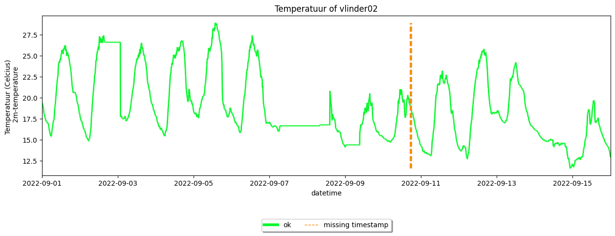
as mentioned above, one can apply the same methods to a Station object:
[13]:
favorite_station.make_plot(colorby='label')
[13]:
<Axes: title={'center': 'Temperatuur of vlinder02'}, xlabel='datetime', ylabel='Temperatuur (Celcius) \n 2m-temperature'>
Resampling the time resolution#
Coarsening the time resolution (i.g. frequency) of your data can be done by using the coarsen_time_resolution().
[14]:
your_dataset.coarsen_time_resolution(freq='30T') #'30T' means 30 minutes

your_dataset.df.head()
[14]:
| temp | radiation_temp | humidity | precip | precip_sum | wind_speed | wind_gust | wind_direction | pressure | pressure_at_sea_level | ||
|---|---|---|---|---|---|---|---|---|---|---|---|
| name | datetime | ||||||||||
| vlinder01 | 2022-09-01 00:00:00+00:00 | 18.8 | NaN | 65 | 0.0 | 0.0 | 5.6 | 11.3 | 65 | 101739 | 102005.0 |
| 2022-09-01 00:30:00+00:00 | 18.7 | NaN | 65 | 0.0 | 0.0 | 5.4 | 9.7 | 85 | 101732 | 101999.0 | |
| 2022-09-01 01:00:00+00:00 | 18.4 | NaN | 65 | 0.0 | 0.0 | 5.1 | 8.1 | 55 | 101736 | 102003.0 | |
| 2022-09-01 01:30:00+00:00 | 18.0 | NaN | 65 | 0.0 | 0.0 | 7.1 | 12.9 | 55 | 101736 | 102003.0 | |
| 2022-09-01 02:00:00+00:00 | 17.1 | NaN | 68 | 0.0 | 0.0 | 5.7 | 9.7 | 45 | 101723 | 101990.0 |
Introduction exercise#
For a more detailed reference, you can use this introduction exercise, that was created in the context of the COST FAIRNESS summerschool 2023 in Ghent.