Demo: Analysis

This example is the continuation of the previous example: filling gaps. This example serves as an introduction to the Analysis module. In the MetObs-toolkit there is a Analysis class, that holds some common methods used in research.

To start, we import the demo dataset.

import metobs_toolkit
dataset = metobs_toolkit.Dataset() #Create a new dataset object

#Load the data
dataset.import_data_from_file(
                    template_file=metobs_toolkit.demo_template, #The template file
                    input_data_file=metobs_toolkit.demo_datafile, #The data file
                    input_metadata_file=metobs_toolkit.demo_metadatafile, #The metadata file
                    )

Luchtdruk is present in the datafile, but not found in the template! This column will be ignored.
Neerslagintensiteit is present in the datafile, but not found in the template! This column will be ignored.
Neerslagsom is present in the datafile, but not found in the template! This column will be ignored.
Rukwind is present in the datafile, but not found in the template! This column will be ignored.
Luchtdruk_Zeeniveau is present in the datafile, but not found in the template! This column will be ignored.
Globe Temperatuur is present in the datafile, but not found in the template! This column will be ignored.
The following columns are present in the data file, but not in the template! They are skipped!
 ['Luchtdruk', 'Luchtdruk_Zeeniveau', 'Neerslagintensiteit', 'Globe Temperatuur', 'Neerslagsom', 'Rukwind']
The following columns are found in the metadata, but not in the template and are therefore ignored:
['benaming', 'stad', 'sponsor', 'Network']

Later in this demo we will some landcover information, we extract this for all are stations in the dataset.

#Get LCZ, and landcover fractions will be used later on
_lczseries = dataset.get_LCZ()

Creating an Analysis

The built-in analysis functionality is centered around the Analysis class. This class holds only records that are assumed to be correct. Thus there are no QC outliers or gaps present defined, the data hold by an Analysis is hold in a single dataframe.

We can create an Analysis instance from a Dataset (or from a Station).

analysis = metobs_toolkit.Analysis(Dataholder=dataset)
analysis.get_info()

================================================================================
                            General info of Analysis
================================================================================

  -Number of records: 120960
  -Observation types: ['humidity', 'temp', 'wind_direction', 'wind_speed']
  -Available metadata columns: ['lat', 'lon', 'altitude', 'LCZ', 'school', 'g...
  -Stations: ['vlinder01', 'vlinder02', 'vlinder03', 'vlinder04', 'vlinder05'...
  -All known time-derivatives: ['year', 'month', 'hour', 'minute', 'second', ...

analysis.df.index.get_level_values('datetime').tz

datetime.timezone.utc

We can inspect the stored data from the Analysis.df and Analysis.metadf attributes.

analysis.df.head(10)

		humidity	temp	wind_direction	wind_speed
datetime	name
2022-09-01 00:00:00+00:00	vlinder01	65.0	18.799999	65.0	1.555556
	vlinder02	62.0	19.400000	25.0	0.194444
	vlinder03	65.0	17.000000	115.0	0.333333
	vlinder04	66.0	15.900000	25.0	0.083333
	vlinder05	61.0	21.100000	45.0	1.611111
	vlinder06	65.0	17.700001	95.0	0.138889
	vlinder07	63.0	18.100000	15.0	0.611111
	vlinder08	59.0	19.200001	165.0	0.222222
	vlinder09	63.0	18.000000	55.0	0.888889
	vlinder10	63.0	19.100000	5.0	0.472222

analysis.metadf.head(10)

	lat	lon	altitude	LCZ	school	geometry
name
vlinder01	50.980438	3.815763	NaN	Low plants (LCZ D)	UGent	POINT (3.81576 50.98044)
vlinder02	51.022381	3.709695	NaN	Large lowrise	UGent	POINT (3.7097 51.02238)
vlinder03	51.324581	4.952109	NaN	Open midrise	Heilig Graf	POINT (4.95211 51.32458)
vlinder04	51.335522	4.934732	NaN	Sparsely built	Heilig Graf	POINT (4.93473 51.33552)
vlinder05	51.052654	3.675183	NaN	Water (LCZ G)	Sint-Barbara	POINT (3.67518 51.05265)
vlinder06	51.027100	4.516300	NaN	Scattered Trees (LCZ B)	BimSem	POINT (4.5163 51.0271)
vlinder07	51.030888	4.478445	NaN	Compact midrise	PTS	POINT (4.47845 51.03089)
vlinder08	51.028130	4.477398	NaN	Compact midrise	TSM	POINT (4.4774 51.02813)
vlinder09	50.927166	4.075722	NaN	Scattered Trees (LCZ B)	SMI	POINT (4.07572 50.92717)
vlinder10	50.935555	4.041389	NaN	Compact midrise	SMI	POINT (4.04139 50.93555)

Analysis methods

An overview of the available analysis methods can be seen in the documentation of the Analysis class. The relevant methods depend on your data and your interests. As an example, a demonstration of the filter and diurnal cycle of the demo data.

Filtering data

It is common to filter your data according to specific meteorological phenomena or periods in time. To do this you can use the apply_filter_on_records() method.

NOTE: The filtering will remove data

print(f'The initial number of records: {analysis.df.shape[0]}')

#filter to non-windy afternoons
analysis.apply_filter_on_records('(wind_speed <= 2.5) & (hour > 12) & (hour < 20)')

#We can apply multiple consecutive filterings
analysis.apply_filter_on_records('season=="autumn" | season=="winter"') #Be aware of quotation!


print(f'The number of records after filtering: {analysis.df.shape[0]}')

The initial number of records: 120960
The number of records after filtering: 28536

We can also use the metadata to filter to by using apply_filter_on_metadata() method.

analysis.apply_filter_on_metadata("LCZ == 'Large lowrise'")

Diurnal cycle

To make a diurnal cycle plot of your Analysis use the get_diurnal_statistics() method:

analysis.plot_diurnal_cycle(colorby='name', #each station is plotted, and colored differently
                            obstype = 'humidity',
                                return_data = False,
                                )

<Axes: title={'center': 'Diurnal cycle of humidity grouped per name.'}, xlabel='Diurnal Timestamps (in UTC)', ylabel='humidity (percent)'>

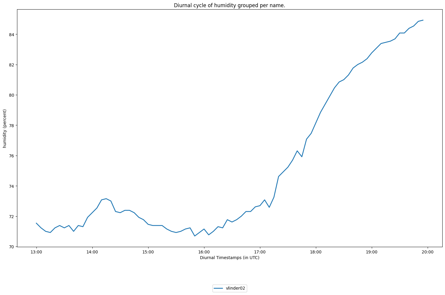
Note: Be aware that we filtered the data to wind-still afternoons in autumn!

If you want to work with the aggregated values, you can use the aggregate_df() method. As illustration we undo the filtering to have some more variability in the data. Then we aggregate the data per LCZ.

import numpy as np

#Start with an unfiltered analysis
analysis=metobs_toolkit.Analysis(Dataholder=dataset)

aggdf = analysis.aggregate_df(
                        obstype='temp',
                        agg=["LCZ", "hour"], #by adding hour, we keep the diurnal variation
                        method=np.mean) #the aggregation function to use.
aggdf

		temp
LCZ	hour
Compact midrise	0	17.739286
	1	17.230398
	2	16.657461
	3	16.421507
	4	16.209682
...	...	...
Water (LCZ G)	19	19.380926
	20	18.933889
	21	18.553888
	22	18.320370
	23	18.126852

240 rows × 1 columns

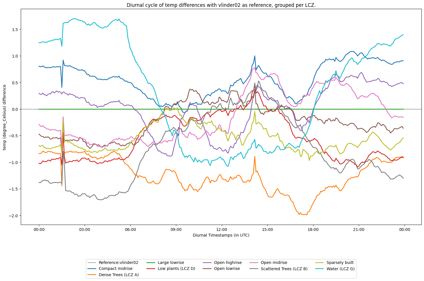
Diurnal cycle of differences

The diurnal cycle of differences is also implemented. The values are the aggregated diurnal differences wrt a reference station.

As an example the diurnal temperature difference cycle is plotted with station vlinder02 as the reference. The aggregation is done per LCZ.

analysis.plot_diurnal_cycle_with_reference_station(ref_station='vlinder02',
                                                  obstype='temp',
                                                  colorby='LCZ')

<Axes: title={'center': 'Diurnal cycle of temp differences with vlinder02 as reference, grouped per LCZ.'}, xlabel='Diurnal Timestamps (in UTC)', ylabel='temp (degree_Celsius) difference'>