Introduction to the MetObs-toolkit

In this introduction, you will learn the principal components and methods in the MetObs-toolkit. Let’s start by importing it.

Since this package is under development, it is often relevant to know the precise version of the toolkit.

import metobs_toolkit

#Print out the version of the toolkit
print(metobs_toolkit.__version__)
import xarray as xr

1.0.0a13

The Dataset class

The Dataset class is for most applications the most important class. It holds all your stations and it’s data. Thus a Dataset is in principal a collection of stations.

Since raw data files often include observations from multiple stations, we import our raw data always directly into a Dataset. We use the Dataset.import_data_from_file() method, to import the raw data into a Dataset.

A key component for importing raw data, is a description of what your data represents and how it is formatted. This is done by providing a template file, that describes how your raw data is structured.

Importing your raw data

As an example we will import a demo file of raw observations. In order to do that we need to :

• Create a template file for our raw data file. The build_template_prompt() function will guide you in this process. It will ask questions, once you answered them a template file is created. It will also propose some code that you use to import your data

• Create a Dataset instance

• Add the raw data into the Dataset.

# Specify the path to your raw data file (we use the demo file as example)
path_to_datafile=metobs_toolkit.demo_datafile

# We will also use a metadata file
path_to_metadatafile=metobs_toolkit.demo_metadatafile

%%script true

#Create a template for these data files
metobs_toolkit.build_template_prompt()

#specify the path to the templatefile that was created
path_to_templatefile=metobs_toolkit.demo_template #demo file as example!!

Now that we have the datafiles and the templatefile, we create an empty Dataset, and import the data into it.

dataset = metobs_toolkit.Dataset() #Create a new dataset object

#Load the data
dataset.import_data_from_file(
                    template_file=path_to_templatefile, #The template file
                    input_data_file=path_to_datafile, #The data file
                    input_metadata_file=path_to_metadatafile, #The metadata file
                    )

Luchtdruk is present in the datafile, but not found in the template! This column will be ignored.
Neerslagintensiteit is present in the datafile, but not found in the template! This column will be ignored.
Neerslagsom is present in the datafile, but not found in the template! This column will be ignored.
Rukwind is present in the datafile, but not found in the template! This column will be ignored.
Luchtdruk_Zeeniveau is present in the datafile, but not found in the template! This column will be ignored.
Globe Temperatuur is present in the datafile, but not found in the template! This column will be ignored.
The following columns are present in the data file, but not in the template! They are skipped!
 ['Luchtdruk', 'Luchtdruk_Zeeniveau', 'Globe Temperatuur', 'Neerslagsom', 'Rukwind', 'Neerslagintensiteit']
The following columns are found in the metadata, but not in the template and are therefore ignored:
['stad', 'benaming', 'sponsor', 'Network']

As can be seen in the printed logs, there is a lot going on when importing the data. That is because tests are applied on your data to check for gaps, and mismatches between data and metadata.

We can now inspect the ´dataset´ further.

The attributes

The attributes are holding the data of the dataset. Here we present some attributes that can be useful to inspect.

All classes in the MetObs-toolkit have a get_info() methods that prints out an overview of its content.

• Dataset.obstypes : A collection of Obstypes that are known. These observationtypes describe a measurable quantity, and its corresponding units.

dataset.obstypes

{'temp': Obstype(id=temp_degree_Celsius),
 'humidity': Obstype(id=humidity_percent),
 'radiation_temp': Obstype(id=radiation_temp_degree_Celsius),
 'pressure': Obstype(id=pressure_hectopascal),
 'pressure_at_sea_level': Obstype(id=pressure_at_sea_level_hectopascal),
 'precip': Obstype(id=precip_millimeter / meter ** 2),
 'precip_sum': Obstype(id=precip_sum_millimeter / meter ** 2),
 'wind_speed': Obstype(id=wind_speed_meter / second),
 'wind_gust': Obstype(id=wind_gust_meter / second),
 'wind_direction': Obstype(id=wind_direction_degree)}

#Note! The known obstypes are NOT the obstypes for which there are observations.
#To get the obstypes for which there are observations, use:
dataset.present_observations

['humidity', 'temp', 'wind_direction', 'wind_speed']

• Dataset.template: A template class, that is automatically set up by using the template file. This is only used when data is imported from a file. It has no further use.

template = dataset.template

template.get_info() # Prints out how the template maps raw data

================================================================================
                            General info of Template
================================================================================


--- Data obstypes map ---

  -temp: Temperatuur
    -raw data in degC
    -description: 2mT passive
  -humidity: Vochtigheid
    -raw data in percent
    -description: 2m relative humidity passive
  -wind_speed: Windsnelheid
    -raw data in km/h
    -description: Average 2m  10-min windspeed
  -wind_direction: Windrichting
    -raw data in degrees
    -description: Average 2m  10-min windspeed, north is zero in CW direction...

--- Data extra mapping info ---

  -name column (data) <---> Vlinder

--- Data timestamp map ---

  -datetimecolumn <---> None
  -time_column <---> Tijd (UTC)
  -date_column <---> Datum
  -fmt <---> %Y-%m-%d %H:%M:%S
  -Timezone <---> UTC

--- Metadata map ---

  -name <---> Vlinder
  -lat <---> lat
  -lon <---> lon
  -school <---> school

• dataset.df: A pandas DataFrame holding all the observation records.

dataset.df

			value	label
datetime	obstype	name
2022-09-01 00:00:00+00:00	humidity	vlinder01	65.000000	ok
		vlinder02	62.000000	ok
		vlinder03	65.000000	ok
		vlinder04	66.000000	ok
		vlinder05	61.000000	ok
...	...	...	...	...
2022-09-15 23:55:00+00:00	wind_speed	vlinder24	0.000000	ok
		vlinder25	1.972222	ok
		vlinder26	0.027778	ok
		vlinder27	0.000000	ok
		vlinder28	0.000000	ok

483840 rows × 2 columns

• dataset.metadf: A pandas DataFrame holding all the metadata of the stations.

dataset.metadf

	lat	lon	altitude	LCZ	school	geometry
name
vlinder01	50.980438	3.815763	NaN	NaN	UGent	POINT (3.81576 50.98044)
vlinder02	51.022381	3.709695	NaN	NaN	UGent	POINT (3.7097 51.02238)
vlinder03	51.324581	4.952109	NaN	NaN	Heilig Graf	POINT (4.95211 51.32458)
vlinder04	51.335522	4.934732	NaN	NaN	Heilig Graf	POINT (4.93473 51.33552)
vlinder05	51.052654	3.675183	NaN	NaN	Sint-Barbara	POINT (3.67518 51.05265)
vlinder06	51.027100	4.516300	NaN	NaN	BimSem	POINT (4.5163 51.0271)
vlinder07	51.030888	4.478445	NaN	NaN	PTS	POINT (4.47845 51.03089)
vlinder08	51.028130	4.477398	NaN	NaN	TSM	POINT (4.4774 51.02813)
vlinder09	50.927166	4.075722	NaN	NaN	SMI	POINT (4.07572 50.92717)
vlinder10	50.935555	4.041389	NaN	NaN	SMI	POINT (4.04139 50.93555)
vlinder11	51.222424	4.381726	NaN	NaN	Sint-Annacollege	POINT (4.38173 51.22242)
vlinder12	51.216476	4.423440	NaN	NaN	UGent	POINT (4.42344 51.21648)
vlinder13	51.212212	4.398065	NaN	NaN	UGent	POINT (4.39807 51.21221)
vlinder14	51.350616	4.315013	NaN	NaN	UGent	POINT (4.31501 51.35062)
vlinder15	50.935299	4.192600	NaN	NaN	Sint-Martinus	POINT (4.1926 50.9353)
vlinder16	51.266850	4.293436	NaN	NaN	Sint-Maarten	POINT (4.29344 51.26685)
vlinder17	51.065269	5.613458	NaN	NaN	Sint-Augustinusinstituut Bree	POINT (5.61346 51.06527)
vlinder18	51.136246	5.656769	NaN	NaN	TISM Bree	POINT (5.65677 51.13625)
vlinder19	50.841454	4.363672	NaN	NaN	UGent	POINT (4.36367 50.84145)
vlinder20	50.847027	4.357971	NaN	NaN	UGent	POINT (4.35797 50.84703)
vlinder21	51.260387	2.991917	NaN	NaN	Zeelyceum	POINT (2.99192 51.26039)
vlinder22	50.989502	2.856220	NaN	NaN	‘t Saam	POINT (2.85622 50.9895)
vlinder23	51.260578	3.580151	NaN	NaN	Richtpunt Eeklo	POINT (3.58015 51.26058)
vlinder24	51.167015	3.572062	NaN	NaN	OLV ten Doorn	POINT (3.57206 51.16702)
vlinder25	51.154720	3.708611	NaN	NaN	Einstein Atheneum	POINT (3.70861 51.15472)
vlinder26	51.161758	4.997653	NaN	NaN	Sint Dimpna	POINT (4.99765 51.16176)
vlinder27	51.058098	3.728067	NaN	NaN	Sec. Kunstinstituut	POINT (3.72807 51.0581)
vlinder28	51.035294	3.769741	NaN	NaN	GO! Ath.	POINT (3.76974 51.03529)

Station class

The stationclass is a representatio of a station. A station holds the following:

• Station.sensordata: Timeseries of an observation type. A station can hold multiple sensordata, one for each sensor.

• Station.site: Each station has a ´Site´ attribute, that holds the information on the location of the station. Metadata related to the station is also stored here.

• Station.modeldata: In addition to the observations, modeldata timeseries representing the station can be stored. In pracktice, if one would download ERA5 data (using the MetObs-toolkit), the timeseries are stored as modeldata in the Station.

To select a station, one can use the name of the station, which is assumed to be unique for each station.

All the methods and attributes that are present in the Dataset are also applicable on the Station! Thus if your script works on Dataset-level, it also works on station-level.

Only the Dataset.sync_records(), Dataset.buddy_check(), and trivial Dataset-only methods (i.g. Dataset.get_station()) are not defined for Stations.

#Select a station
your_station = dataset.get_station('vlinder02')

#Print out some details
your_station.get_info()

================================================================================
                            General info of Station
================================================================================


--- Observational info ---

Station instance with:
  -humidity:
    -humidity observations in percent
    -from 2022-09-01 00:00:00+00:00 -> 2022-09-15 23:55:00+00:00
    -At a resolution of 0 days 00:05:00
    -No outliers present.
    -2 gaps present, a total of 3 missing timestamps.
      -label counts:
        -gap: 3
  -temp:
    -temp observations in degree_Celsius
    -from 2022-09-01 00:00:00+00:00 -> 2022-09-15 23:55:00+00:00
    -At a resolution of 0 days 00:05:00
    -No outliers present.
    -2 gaps present, a total of 3 missing timestamps.
      -label counts:
        -gap: 3
  -wind_direction:
    -wind_direction observations in degree
    -from 2022-09-01 00:00:00+00:00 -> 2022-09-15 23:55:00+00:00
    -At a resolution of 0 days 00:05:00
    -No outliers present.
    -2 gaps present, a total of 3 missing timestamps.
      -label counts:
        -gap: 3
  -wind_speed:
    -wind_speed observations in meter / second
    -from 2022-09-01 00:00:00+00:00 -> 2022-09-15 23:55:00+00:00
    -At a resolution of 0 days 00:05:00
    -No outliers present.
    -2 gaps present, a total of 3 missing timestamps.
      -label counts:
        -gap: 3

--- Metadata info ---

  -Coordinates (51.022379, 3.709695) (latitude, longitude)
  -Altitude is unknown
  -LCZ is unknown
  -Land cover fractions are unknown
  -Extra metadata from the metadata file:
    -school: UGent

--- Modeldata info ---

  -Station instance without model data.

# Inspecting the attributes of the station

#Print out info on the Site of the station:
your_station.site.get_info()

================================================================================
                              General Info of Site
================================================================================

Site of vlinder02:
  -Coordinates (51.022379, 3.709695) (latitude, longitude)
  -Altitude is unknown
  -LCZ is unknown
  -Land cover fractions are unknown
  -Extra metadata from the metadata file:
    -school: UGent

# All observational data is stored as SensorData

print(your_station.get_sensor('temp'))

# More convenient is to use the pandas dataframe representations,
# similar as with the Dataset

your_station.df

temp data of station vlinder02.

		value	label
datetime	obstype
2022-09-01 00:00:00+00:00	humidity	62.000000	ok
	temp	19.400000	ok
	wind_direction	25.000000	ok
	wind_speed	0.194444	ok
2022-09-01 00:05:00+00:00	humidity	62.000000	ok
...	...	...	...
2022-09-15 23:50:00+00:00	wind_speed	0.000000	ok
2022-09-15 23:55:00+00:00	humidity	83.000000	ok
	temp	12.900000	ok
	wind_direction	295.000000	ok
	wind_speed	0.000000	ok

17280 rows × 2 columns

#Or the metadata for this singel station
your_station.metadf

	lat	lon	altitude	LCZ	school	geometry
name
vlinder02	51.022381	3.709695	NaN	NaN	UGent	POINT (3.7097 51.02238)

Plotting timeseries

Plotting the timeseries can be simply done by using the make_plot() method, on a Dataset or a Station.

dataset.make_plot(obstype='temp', #Which observation type to plot. (See dataset.present_observations)
                  colorby='station', #if 'station', each station will be a different color
                  show_outliers=True,
                  show_gaps=True)

<Axes: title={'center': 'temp data.'}, xlabel='Timestamps (in UTC)', ylabel='temp (degree_Celsius)'>

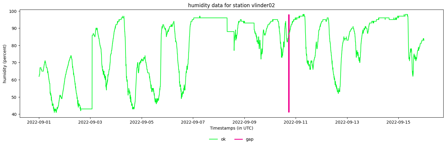
#We can also plot a single station
your_station.make_plot(obstype='humidity',
                       colorby='label') #If 'label', the colors are based on the status/label of an observation.

<Axes: title={'center': 'humidity data for station vlinder02'}, xlabel='Timestamps (in UTC)', ylabel='humidity (percent)'>

Common usecases

Here a collection of common usecases.

Resampling time resolution

It is common to change or alter the time resolution of your observations. This is often applied when:

• the data amount is to big, and the present time resolution is not required for the analysis.

• sensor do not have the same time resolution. (i.g. temperature is measured every 5 minutes, but precipitation is measured each hour.)

• Observations are not synchronized over multiple stations. This is a special case of resampling, since there is also a synchronization required.

It is recommended to set the target time resolution, in the beginning of your pipeline!

In the MetObs-toolkit you can resample by using the resample() method on a Dataset or Station. By doing so, the toolkit will construct a set of target timestamps (in the new resolution), and will map the raw timestamps to the new target timestamps. There is no interpolation applied!

In order to construct the mapping of the old timestamps to the target timestamps, a tolerance is used. The nearest timestamp is tested if it is within the tolerance of the target timestamp. If this test is not successful, no record could be assigned to the target timestamp and thus a gap is created. Thus by increasing the shift_tolerance, the resampling method will have more mapped timestamps thus less gaps but at the cost of less accurate timestamps.

hourly_dataset = metobs_toolkit.Dataset()
#Load the data (raw data has 5 min resolution)
hourly_dataset.import_data_from_file(
                    template_file=path_to_templatefile, #The template file
                    input_data_file=path_to_datafile, #The data file
                    input_metadata_file=path_to_metadatafile, #The metadata file
                    )
#Resample to 1 hour resolution
hourly_dataset.resample(target_freq='1h', #Target frequency is set to 1 hour
                        obstype=None, #if None, all present observations are resampled
                        shift_tolerance='4min', #The maximum shift allow for a timestamp
                        origin_simplify_tolerance='3min') # The maximum shift for the origin, to get a simplified origin

# You can verify that the resolution is hourly by inspecting the df attribute
hourly_dataset.df.index

WARNING:<metobs_toolkit>:Luchtdruk is present in the datafile, but not found in the template! This column will be ignored.
WARNING:<metobs_toolkit>:Neerslagintensiteit is present in the datafile, but not found in the template! This column will be ignored.
WARNING:<metobs_toolkit>:Neerslagsom is present in the datafile, but not found in the template! This column will be ignored.
WARNING:<metobs_toolkit>:Rukwind is present in the datafile, but not found in the template! This column will be ignored.
WARNING:<metobs_toolkit>:Luchtdruk_Zeeniveau is present in the datafile, but not found in the template! This column will be ignored.
WARNING:<metobs_toolkit>:Globe Temperatuur is present in the datafile, but not found in the template! This column will be ignored.
WARNING:<metobs_toolkit>:The following columns are present in the data file, but not in the template! They are skipped!
 ['Luchtdruk', 'Luchtdruk_Zeeniveau', 'Globe Temperatuur', 'Neerslagsom', 'Rukwind', 'Neerslagintensiteit']
WARNING:<metobs_toolkit>:The following columns are found in the metadata, but not in the template and are therefore ignored:
['stad', 'benaming', 'sponsor', 'Network']
WARNING:<metobs_toolkit>:The present gaps are removed, new gaps are constructed for temp data of station vlinder02..
WARNING:<metobs_toolkit>:The present gaps are removed, new gaps are constructed for wind_direction data of station vlinder02..
WARNING:<metobs_toolkit>:The present gaps are removed, new gaps are constructed for wind_speed data of station vlinder02..
WARNING:<metobs_toolkit>:The present gaps are removed, new gaps are constructed for humidity data of station vlinder02..

MultiIndex([('2022-09-01 00:00:00+00:00',   'humidity', 'vlinder01'),
            ('2022-09-01 00:00:00+00:00',   'humidity', 'vlinder02'),
            ('2022-09-01 00:00:00+00:00',   'humidity', 'vlinder03'),
            ('2022-09-01 00:00:00+00:00',   'humidity', 'vlinder04'),
            ('2022-09-01 00:00:00+00:00',   'humidity', 'vlinder05'),
            ('2022-09-01 00:00:00+00:00',   'humidity', 'vlinder06'),
            ('2022-09-01 00:00:00+00:00',   'humidity', 'vlinder07'),
            ('2022-09-01 00:00:00+00:00',   'humidity', 'vlinder08'),
            ('2022-09-01 00:00:00+00:00',   'humidity', 'vlinder09'),
            ('2022-09-01 00:00:00+00:00',   'humidity', 'vlinder10'),
            ...
            ('2022-09-15 23:00:00+00:00', 'wind_speed', 'vlinder19'),
            ('2022-09-15 23:00:00+00:00', 'wind_speed', 'vlinder20'),
            ('2022-09-15 23:00:00+00:00', 'wind_speed', 'vlinder21'),
            ('2022-09-15 23:00:00+00:00', 'wind_speed', 'vlinder22'),
            ('2022-09-15 23:00:00+00:00', 'wind_speed', 'vlinder23'),
            ('2022-09-15 23:00:00+00:00', 'wind_speed', 'vlinder24'),
            ('2022-09-15 23:00:00+00:00', 'wind_speed', 'vlinder25'),
            ('2022-09-15 23:00:00+00:00', 'wind_speed', 'vlinder26'),
            ('2022-09-15 23:00:00+00:00', 'wind_speed', 'vlinder27'),
            ('2022-09-15 23:00:00+00:00', 'wind_speed', 'vlinder28')],
           names=['datetime', 'obstype', 'name'], length=40320)

Dataframe of one observationtype

The Dataset.df and Station.df returns a pandas dataframe with a so called Multi-Index. That is because the combination of [´timestamp´, ´observationtype´, ‘stationname´] defines an observation, thus the use of the Multi-Index.

We are aware that working with Multi-Indexed dataframes can be challenging, thus an example on how to convert a multiindex dataframe to a regular-indexed dataframe.

Be aware that removing (or reducing) the Multi-Index, is always a subsetting or approximation.

#Subset to only temperatures (=subsetting)

temperatures = dataset.df.xs(key='temp',
                             level='obstype', #the level of the index ('datetime', 'name' or 'obstype')
                             drop_level=True)

#You can see that the index now only has 2-levels:
temperatures

		value	label
datetime	name
2022-09-01 00:00:00+00:00	vlinder01	18.799999	ok
	vlinder02	19.400000	ok
	vlinder03	17.000000	ok
	vlinder04	15.900000	ok
	vlinder05	21.100000	ok
...	...	...	...
2022-09-15 23:55:00+00:00	vlinder24	11.100000	ok
	vlinder25	14.100000	ok
	vlinder26	13.300000	ok
	vlinder27	14.300000	ok
	vlinder28	13.000000	ok

120960 rows × 2 columns

#If we assume that all the temperature observations over all the stations have the same
#set of timestamps (typical after resampling! ), we can create a dataframe with all stations represented by columns.

temperatures_wide = (dataset.df
                    #first subset to temperatures
                    .xs(key='temp',
                            level='obstype', #the level of the index ('datetime', 'name' or 'obstype')
                            drop_level=True)
                    #Convert a index level to columns (unstacking)
                    .unstack(level='name'))
temperatures_wide

	value										...	label
name	vlinder01	vlinder02	vlinder03	vlinder04	vlinder05	vlinder06	vlinder07	vlinder08	vlinder09	vlinder10	...	vlinder19	vlinder20	vlinder21	vlinder22	vlinder23	vlinder24	vlinder25	vlinder26	vlinder27	vlinder28
datetime
2022-09-01 00:00:00+00:00	18.799999	19.400000	17.000000	15.9	21.1	17.700001	18.1	19.200001	18.000000	19.100000	...	ok	ok	ok	ok	ok	ok	ok	ok	ok	ok
2022-09-01 00:05:00+00:00	18.799999	19.400000	16.900000	15.8	21.1	17.700001	18.1	19.100000	18.000000	19.000000	...	ok	ok	ok	ok	ok	ok	ok	ok	ok	ok
2022-09-01 00:10:00+00:00	18.799999	19.299999	16.799999	15.8	21.1	17.600000	18.0	19.100000	17.900000	18.900000	...	ok	ok	ok	ok	ok	ok	ok	ok	ok	ok
2022-09-01 00:15:00+00:00	18.700001	19.200001	16.700001	15.6	21.1	17.500000	18.0	19.000000	17.799999	18.900000	...	ok	ok	ok	ok	ok	ok	ok	ok	ok	ok
2022-09-01 00:20:00+00:00	18.700001	19.200001	16.600000	15.4	21.1	17.500000	18.1	19.000000	17.700001	18.799999	...	ok	ok	ok	ok	ok	ok	ok	ok	ok	ok
...	...	...	...	...	...	...	...	...	...	...	...	...	...	...	...	...	...	...	...	...	...
2022-09-15 23:35:00+00:00	13.200000	13.300000	12.200000	9.1	17.4	13.200000	13.4	14.400000	13.200000	14.300000	...	ok	ok	ok	ok	ok	ok	ok	ok	ok	ok
2022-09-15 23:40:00+00:00	13.100000	13.200000	12.200000	9.6	17.4	13.100000	13.4	14.300000	13.100000	14.200000	...	ok	ok	ok	ok	ok	ok	ok	ok	ok	ok
2022-09-15 23:45:00+00:00	13.000000	13.100000	12.200000	9.8	17.4	13.000000	13.3	14.300000	13.000000	14.200000	...	ok	ok	ok	ok	ok	ok	ok	ok	ok	ok
2022-09-15 23:50:00+00:00	12.900000	13.000000	12.300000	10.0	17.4	13.100000	13.3	14.200000	13.000000	14.200000	...	ok	ok	ok	ok	ok	ok	ok	ok	ok	ok
2022-09-15 23:55:00+00:00	12.900000	12.900000	12.400000	10.2	17.4	13.100000	13.2	14.200000	13.000000	14.100000	...	ok	ok	ok	ok	ok	ok	ok	ok	ok	ok

4320 rows × 56 columns

#if you are only interested in the value, you can select them:
temperatures_wide['value']

name	vlinder01	vlinder02	vlinder03	vlinder04	vlinder05	vlinder06	vlinder07	vlinder08	vlinder09	vlinder10	...	vlinder19	vlinder20	vlinder21	vlinder22	vlinder23	vlinder24	vlinder25	vlinder26	vlinder27	vlinder28
datetime
2022-09-01 00:00:00+00:00	18.799999	19.400000	17.000000	15.9	21.1	17.700001	18.1	19.200001	18.000000	19.100000	...	18.700001	19.400000	19.299999	18.799999	18.0	18.200001	18.900000	17.900000	19.600000	17.799999
2022-09-01 00:05:00+00:00	18.799999	19.400000	16.900000	15.8	21.1	17.700001	18.1	19.100000	18.000000	19.000000	...	18.600000	19.400000	19.299999	18.799999	18.0	18.200001	18.500000	17.700001	19.600000	17.799999
2022-09-01 00:10:00+00:00	18.799999	19.299999	16.799999	15.8	21.1	17.600000	18.0	19.100000	17.900000	18.900000	...	18.600000	19.299999	19.200001	18.700001	18.0	18.100000	18.299999	17.500000	19.500000	17.700001
2022-09-01 00:15:00+00:00	18.700001	19.200001	16.700001	15.6	21.1	17.500000	18.0	19.000000	17.799999	18.900000	...	18.500000	19.299999	19.200001	18.600000	18.0	18.000000	18.200001	17.299999	19.400000	17.799999
2022-09-01 00:20:00+00:00	18.700001	19.200001	16.600000	15.4	21.1	17.500000	18.1	19.000000	17.700001	18.799999	...	18.500000	19.200001	19.200001	18.299999	18.0	17.900000	18.100000	17.100000	19.299999	17.799999
...	...	...	...	...	...	...	...	...	...	...	...	...	...	...	...	...	...	...	...	...	...
2022-09-15 23:35:00+00:00	13.200000	13.300000	12.200000	9.1	17.4	13.200000	13.4	14.400000	13.200000	14.300000	...	14.500000	15.000000	15.700000	12.100000	13.9	11.700000	14.200000	13.400000	14.500000	13.400000
2022-09-15 23:40:00+00:00	13.100000	13.200000	12.200000	9.6	17.4	13.100000	13.4	14.300000	13.100000	14.200000	...	14.500000	15.000000	15.700000	12.100000	13.9	11.600000	14.200000	13.400000	14.500000	13.300000
2022-09-15 23:45:00+00:00	13.000000	13.100000	12.200000	9.8	17.4	13.000000	13.3	14.300000	13.000000	14.200000	...	14.400000	14.900000	15.600000	12.100000	13.8	11.400000	14.200000	13.400000	14.400000	13.200000
2022-09-15 23:50:00+00:00	12.900000	13.000000	12.300000	10.0	17.4	13.100000	13.3	14.200000	13.000000	14.200000	...	14.300000	14.900000	15.700000	12.000000	13.9	11.300000	14.200000	13.400000	14.400000	13.200000
2022-09-15 23:55:00+00:00	12.900000	12.900000	12.400000	10.2	17.4	13.100000	13.2	14.200000	13.000000	14.100000	...	14.300000	14.800000	15.600000	11.900000	13.9	11.100000	14.100000	13.300000	14.300000	13.000000

4320 rows × 28 columns

Exporting data

The MetObs-toolkit provides several methods to export your processed data in different formats, each serving different purposes:

For data analysis and interoperability:

• to_parquet() and to_csv() export the observation data as flat tables, ideal for analysis in other tools

• to_xr() converts the dataset to an xarray Dataset.

These methods can be applied on a Dataset and on a Station.

For preserving the complete MetObs-toolkit structure:

• save_dataset_to_pkl() saves the entire Dataset object including all metadata, QC flags, and internal structures

The key difference is that save_dataset_to_pkl() preserves the complete MetObs-toolkit Dataset structure and can be reloaded with load_dataset_from_pkl(), while the other methods export only the observation data in standard formats for external use.

# Export the entire dataset to parquet format
dataset.to_parquet("my_dataset.parquet", overwrite=True)

# Export the entire dataset to CSV format
dataset.to_csv("my_dataset.csv", overwrite=True)

# Export the dataset to netCDF
dataset.to_netcdf("my_dataset.nc", overwrite=True)

# Convert the entire dataset to an xarray Dataset
xr_dataset = dataset.to_xr()
xr_dataset

<xarray.Dataset> Size: 8MB
Dimensions:         (name: 28, kind: 2, datetime: 4320)
Coordinates:
  * name            (name) <U9 1kB 'vlinder01' 'vlinder02' ... 'vlinder28'
    lat             (name) float64 224B 50.98 51.02 51.32 ... 51.16 51.06 51.04
    lon             (name) float64 224B 3.816 3.71 4.952 ... 4.998 3.728 3.77
    school          (name) <U29 3kB 'UGent' 'UGent' ... 'GO! Ath.'
  * kind            (kind) <U5 40B 'obs' 'label'
  * datetime        (datetime) datetime64[ns] 35kB 2022-09-01 ... 2022-09-15T...
    altitude        float64 8B nan
    LCZ             float64 8B nan
Data variables:
    temp            (name, kind, datetime) float64 2MB 18.8 18.8 ... 0.0 0.0
    wind_direction  (name, kind, datetime) float64 2MB 65.0 75.0 ... 0.0 0.0
    wind_speed      (name, kind, datetime) float64 2MB 1.556 1.528 ... 0.0 0.0
    humidity        (name, kind, datetime) float64 2MB 65.0 65.0 ... 0.0 0.0

xarray.Dataset

• Dimensions:
  • name: 28
  • kind: 2
  • datetime: 4320
• Coordinates: (8)
  • name
    (name)
    <U9
    'vlinder01' ... 'vlinder28'

    array(['vlinder01', 'vlinder02', 'vlinder03', 'vlinder04', 'vlinder05',
           'vlinder06', 'vlinder07', 'vlinder08', 'vlinder09', 'vlinder10',
           'vlinder11', 'vlinder12', 'vlinder13', 'vlinder14', 'vlinder15',
           'vlinder16', 'vlinder17', 'vlinder18', 'vlinder19', 'vlinder20',
           'vlinder21', 'vlinder22', 'vlinder23', 'vlinder24', 'vlinder25',
           'vlinder26', 'vlinder27', 'vlinder28'], dtype='<U9')

  • lat
    (name)
    float64
    50.98 51.02 51.32 ... 51.06 51.04

    array([50.980438, 51.022379, 51.324583, 51.335522, 51.052655, 51.0271  ,
           51.030889, 51.02813 , 50.927167, 50.935556, 51.222422, 51.216477,
           51.212211, 51.350618, 50.9353  , 51.26685 , 51.065269, 51.136244,
           50.841455, 50.847025, 51.260389, 50.989501, 51.260578, 51.167015,
           51.15472 , 51.16176 , 51.058099, 51.035293])

  • lon
    (name)
    float64
    3.816 3.71 4.952 ... 3.728 3.77

    array([3.815763, 3.709695, 4.952109, 4.934732, 3.675183, 4.5163  ,
           4.478445, 4.477398, 4.075722, 4.041389, 4.381726, 4.42344 ,
           4.398065, 4.315013, 4.1926  , 4.293436, 5.613458, 5.656769,
           4.363672, 4.357971, 2.991917, 2.85622 , 3.580151, 3.572062,
           3.708611, 4.997653, 3.728067, 3.769741])

  • school
    (name)
    <U29
    'UGent' 'UGent' ... 'GO! Ath.'

    array(['UGent', 'UGent', 'Heilig Graf', 'Heilig Graf', 'Sint-Barbara',
           'BimSem', 'PTS', 'TSM', 'SMI', 'SMI', 'Sint-Annacollege', 'UGent',
           'UGent', 'UGent', 'Sint-Martinus', 'Sint-Maarten',
           'Sint-Augustinusinstituut Bree', 'TISM Bree', 'UGent', 'UGent',
           'Zeelyceum', '‘t Saam', 'Richtpunt Eeklo', 'OLV ten Doorn',
           'Einstein Atheneum', 'Sint Dimpna', 'Sec. Kunstinstituut',
           'GO! Ath.'], dtype='<U29')

  • kind
    (kind)
    <U5
    'obs' 'label'

    array(['obs', 'label'], dtype='<U5')

  • datetime
    (datetime)
    datetime64[ns]
    2022-09-01 ... 2022-09-15T23:55:00

    timezone :

    UTC

    standard_name :

    time

    long_name :

    time

    array(['2022-09-01T00:00:00.000000000', '2022-09-01T00:05:00.000000000',
           '2022-09-01T00:10:00.000000000', ..., '2022-09-15T23:45:00.000000000',
           '2022-09-15T23:50:00.000000000', '2022-09-15T23:55:00.000000000'],
          shape=(4320,), dtype='datetime64[ns]')

  • altitude
    ()
    float64
    nan

    array(nan)

  • LCZ
    ()
    float64
    nan

    array(nan)

• Data variables: (4)
  • temp
    (name, kind, datetime)
    float64
    18.8 18.8 18.8 18.7 ... 0.0 0.0 0.0

    obstype_name :

    temp

    obstype_desc :

    2m - temperature

    obstype_unit :

    degree_Celsius

    MetObs toolkit version :

    1.0.0a13

    QC checks :

    ['duplicated_timestamp']

    GF methods :

    []

    Label:ok :

    0

    array([[[18.79999924, 18.79999924, 18.79999924, ..., 13.        ,
             12.89999962, 12.89999962],
            [ 0.        ,  0.        ,  0.        , ...,  0.        ,
              0.        ,  0.        ]],
    
           [[19.39999962, 19.39999962, 19.29999924, ..., 13.10000038,
             13.        , 12.89999962],
            [ 0.        ,  0.        ,  0.        , ...,  0.        ,
              0.        ,  0.        ]],
    
           [[17.        , 16.89999962, 16.79999924, ..., 12.19999981,
             12.30000019, 12.39999962],
            [ 0.        ,  0.        ,  0.        , ...,  0.        ,
              0.        ,  0.        ]],
    
           ...,
    
           [[17.89999962, 17.70000076, 17.5       , ..., 13.39999962,
             13.39999962, 13.30000019],
            [ 0.        ,  0.        ,  0.        , ...,  0.        ,
              0.        ,  0.        ]],
    
           [[19.60000038, 19.60000038, 19.5       , ..., 14.39999962,
             14.39999962, 14.30000019],
            [ 0.        ,  0.        ,  0.        , ...,  0.        ,
              0.        ,  0.        ]],
    
           [[17.79999924, 17.79999924, 17.70000076, ..., 13.19999981,
             13.19999981, 13.        ],
            [ 0.        ,  0.        ,  0.        , ...,  0.        ,
              0.        ,  0.        ]]], shape=(28, 2, 4320))

  • wind_direction
    (name, kind, datetime)
    float64
    65.0 75.0 75.0 85.0 ... 0.0 0.0 0.0

    obstype_name :

    wind_direction

    obstype_desc :

    wind direction

    obstype_unit :

    degree

    MetObs toolkit version :

    1.0.0a13

    QC checks :

    ['duplicated_timestamp']

    GF methods :

    []

    Label:ok :

    0

    array([[[ 65.,  75.,  75., ..., 295., 295., 295.],
            [  0.,   0.,   0., ...,   0.,   0.,   0.]],
    
           [[ 25.,  85.,  45., ..., 295., 295., 295.],
            [  0.,   0.,   0., ...,   0.,   0.,   0.]],
    
           [[115., 115., 115., ...,  95.,  85.,  85.],
            [  0.,   0.,   0., ...,   0.,   0.,   0.]],
    
           ...,
    
           [[355.,  25.,  15., ...,   5.,   5.,   5.],
            [  0.,   0.,   0., ...,   0.,   0.,   0.]],
    
           [[335., 335., 335., ...,  85.,  85.,  85.],
            [  0.,   0.,   0., ...,   0.,   0.,   0.]],
    
           [[115., 115.,  35., ..., 275., 275., 285.],
            [  0.,   0.,   0., ...,   0.,   0.,   0.]]], shape=(28, 2, 4320))

  • wind_speed
    (name, kind, datetime)
    float64
    1.556 1.528 1.417 ... 0.0 0.0 0.0

    obstype_name :

    wind_speed

    obstype_desc :

    wind speed

    obstype_unit :

    meter / second

    MetObs toolkit version :

    1.0.0a13

    QC checks :

    ['duplicated_timestamp']

    GF methods :

    []

    Label:ok :

    0

    array([[[1.55555558, 1.52777791, 1.41666675, ..., 0.08333334,
             0.30555558, 0.11111112],
            [0.        , 0.        , 0.        , ..., 0.        ,
             0.        , 0.        ]],
    
           [[0.19444445, 0.11111112, 0.25      , ..., 0.        ,
             0.        , 0.        ],
            [0.        , 0.        , 0.        , ..., 0.        ,
             0.        , 0.        ]],
    
           [[0.33333337, 0.30555558, 0.27777779, ..., 0.16666669,
             0.02777778, 0.        ],
            [0.        , 0.        , 0.        , ..., 0.        ,
             0.        , 0.        ]],
    
           ...,
    
           [[0.88888896, 0.97222227, 0.72222221, ..., 0.05555556,
             0.        , 0.02777778],
            [0.        , 0.        , 0.        , ..., 0.        ,
             0.        , 0.        ]],
    
           [[0.        , 0.        , 0.        , ..., 0.        ,
             0.        , 0.        ],
            [0.        , 0.        , 0.        , ..., 0.        ,
             0.        , 0.        ]],
    
           [[0.        , 0.        , 0.25      , ..., 0.        ,
             0.        , 0.        ],
            [0.        , 0.        , 0.        , ..., 0.        ,
             0.        , 0.        ]]], shape=(28, 2, 4320))

  • humidity
    (name, kind, datetime)
    float64
    65.0 65.0 65.0 65.0 ... 0.0 0.0 0.0

    obstype_name :

    humidity

    obstype_desc :

    2m - relative humidity

    obstype_unit :

    percent

    MetObs toolkit version :

    1.0.0a13

    QC checks :

    ['duplicated_timestamp']

    GF methods :

    []

    Label:ok :

    0

    array([[[65., 65., 65., ..., 87., 86., 86.],
            [ 0.,  0.,  0., ...,  0.,  0.,  0.]],
    
           [[62., 62., 62., ..., 83., 83., 83.],
            [ 0.,  0.,  0., ...,  0.,  0.,  0.]],
    
           [[65., 65., 65., ..., 78., 78., 77.],
            [ 0.,  0.,  0., ...,  0.,  0.,  0.]],
    
           ...,
    
           [[61., 61., 62., ..., 77., 78., 77.],
            [ 0.,  0.,  0., ...,  0.,  0.,  0.]],
    
           [[60., 60., 61., ..., 71., 71., 71.],
            [ 0.,  0.,  0., ...,  0.,  0.,  0.]],
    
           [[69., 69., 69., ..., 77., 77., 77.],
            [ 0.,  0.,  0., ...,  0.,  0.,  0.]]], shape=(28, 2, 4320))

Quality control

For more details, refer to the Quality Control Example Notebook.

Extracting data from Google Earth Engine

For an introduction to extracting data for GEE, we refer to the Using Google Earth Engine demo.

Filling gaps

For an introduction to filling gaps, we refer to the Filling gaps demo.

Analysis

For an introduction to analyzing your dataset, we refer to the Analysis demo.