Demo: Using Google Earth engine#
This example serves as a demonstration on how to interact with Google Earth Engine (GEE) from within the MetObs-toolkit framework.
[1]:
import metobs_toolkit
GEE authentication#
Before proceeding, make sure you have set up a Google developers account and a GEE project. See Using Google Earth Engine for a detailed description of this.
To test the GEE authentication we can use the metobs_toolkit.connect_to_gee method. If you authenticate using new credentials, make sure NOT to check the read-only-scopes. (See Extracting ERA5 data).
[2]:
%%script true

metobs_toolkit.connect_to_gee() #Uses a credetial file that is stored on your computer
If something is wrong with your credential (or it is the first time/ expiered credetials) you can force the creation of a new credential (file). You only need to run this if the metobs_toolkit.connect_to_gee() returned an error.
[3]:
%%script true

metobs_toolkit.connect_to_gee(
    force=True, #create new credentials
    auth_mode='notebook', # 'notebook', 'localhost', 'gcloud' (requires gcloud installed) or 'colab' (works only in colab)
)
For more details on authentication we refer to the Using Google Earth Engine <../Using_gee.html>_ page and the authentication info page of GEE.
GEE interaction from the MetObs-toolkit#
There are two classes that facilitate the interaction with GEE and the metobs_toolkit:
GeeStaticDatasetManager: This class handles GEE Datasets that do not have a time dimension (static).GeeDynamicDatasetManager: This class handles GEE Datasets that have a time dimension.
Both classes holds all the information to extract data, at the location of your stations, from the corresponding GEE dataset. For the GeeStaticDatasetManager the extracted data will update the metadata of the stations and the corresponding Station.site attribute will be update. Typical examples are the extraction of Local Climate Zones (LCZ), altitude and landcoverfractions.
When data is extracted using a GeeDynamicDatasetManager, timeseries is typically extracted. These timeseries are stored in ModelTimeSeries. Typical examples are the extraction of ERA5 equivalent timeseries for a sensor.
By default some a GEEDatasetManager is create for some popular datasets:
[4]:
default_managers=metobs_toolkit.default_GEE_datasets
default_managers
[4]:
{'LCZ': GeeStaticDatasetManager representation of LCZ ,
 'altitude': GeeStaticDatasetManager representation of altitude ,
 'worldcover': GeeStaticDatasetManager representation of worldcover ,
 'ERA5-land': GeeDynamicDatasetManager representation of ERA5-land }
We can see that by default there are 3 GeeStaticDatasetManagers (lcz, altitude and worldcover), and one GeeDynamicDatasetManager (ERA5-land).
Let’s look at the local climate zones (LCZ) dataset manager as example:
[5]:
default_managers['LCZ'].get_info()
================================================================================
                        General info of GEEStaticDataset
================================================================================


--- GEE Dataset details ---

  -name: LCZ
  -location: RUB/RUBCLIM/LCZ/global_lcz_map/latest
  -value_type: categorical
  -scale: 100
  -is_static: True
  -is_image: False
  -is_mosaic: True
  -credentials: Demuzere M.; Kittner J.; Martilli A.; Mills, G.; Moede, C.; S...
  -target band: LCZ_Filter
  -classification:
    -1: Compact highrise
    -2: Compact midrise
    -3: Compact lowrise
    -4: Open highrise
    -5: Open midrise
    -6: Open lowrise
    -7: Lightweight lowrise
    -8: Large lowrise
    -9: Sparsely built
    -10: Heavy industry
    -11: Dense Trees (LCZ A)
    -12: Scattered Trees (LCZ B)
    -13: Bush, scrub (LCZ C)
    -14: Low plants (LCZ D)
    -15: Bare rock or paved (LCZ E)
    -16: Bare soil or sand (LCZ F)
    -17: Water (LCZ G)
  -aggregation:
  -colors:
    -1: #8c0000
    -2: #d10000
    -3: #ff0000
    -4: #bf4d00
    -5: #ff6600
    -6: #ff9955
    -7: #faee05
    -8: #bcbcbc
    -9: #ffccaa
    -10: #555555
    -11: #006a00
    -12: #00aa00
    -13: #648525
    -14: #b9db79
    -15: #000000
    -16: #fbf7ae
    -17: #6a6aff
As you can see, the DatasetManager contains info on where this dataset is stored on GEE, some details on the dataset and some defenitions (color schemes, aggregation, label defenitions).
Extracting data from GEE#
As a demonstration we are going to extract data from GEE. When we use the MetObs-toolkit for it, it will extract data from GEE only at the locations of the stations. This extracted data is thus linked to a station (by location).
Some common pracktices are to get the LCZ, altitude and some landcover information of all the stations. We start by importin the demo data and extract these details from corresponding datasets on GEE.
[6]:
#Import the demo dataset
dataset = metobs_toolkit.Dataset()
dataset.import_data_from_file(
    template_file=metobs_toolkit.demo_template,
    input_data_file=metobs_toolkit.demo_datafile,
    input_metadata_file=metobs_toolkit.demo_metadatafile,
)
Luchtdruk is present in the datafile, but not found in the template! This column will be ignored.
Neerslagintensiteit is present in the datafile, but not found in the template! This column will be ignored.
Neerslagsom is present in the datafile, but not found in the template! This column will be ignored.
Rukwind is present in the datafile, but not found in the template! This column will be ignored.
Luchtdruk_Zeeniveau is present in the datafile, but not found in the template! This column will be ignored.
Globe Temperatuur is present in the datafile, but not found in the template! This column will be ignored.
The following columns are present in the data file, but not in the template! They are skipped!
 ['Luchtdruk_Zeeniveau', 'Luchtdruk', 'Rukwind', 'Neerslagsom', 'Globe Temperatuur', 'Neerslagintensiteit']
The following columns are found in the metadata, but not in the template and are therefore ignored:
['Network', 'sponsor', 'stad', 'benaming']
The current metdata is rather limited:
[7]:
dataset.metadf.head(5)
[7]:
| lat | lon | school | geometry | |
|---|---|---|---|---|
| name | ||||
| vlinder01 | 50.980438 | 3.815763 | UGent | POINT (3.81576 50.98044) |
| vlinder02 | 51.022379 | 3.709695 | UGent | POINT (3.7097 51.02238) |
| vlinder03 | 51.324583 | 4.952109 | Heilig Graf | POINT (4.95211 51.32458) |
| vlinder04 | 51.335522 | 4.934732 | Heilig Graf | POINT (4.93473 51.33552) |
| vlinder05 | 51.052655 | 3.675183 | Sint-Barbara | POINT (3.67518 51.05266) |
To extract geospatial information for your stations, the lat and lon (latitude and longitude) of your stations must be present in the metadf. If so, then geospatial information will be extracted from GEE at these locations.
Extracting LCZ from GEE#
To extract the Local Climate Zones (LCZs) of your stations:
[8]:
LCZ_values = dataset.get_LCZ()

# The LCZs for all your stations are extracted
print(LCZ_values.head(5))
                          LCZ
name
vlinder01  Low plants (LCZ D)
vlinder02       Large lowrise
vlinder03        Open midrise
vlinder04      Sparsely built
vlinder05       Water (LCZ G)
The LCZ data is returned by the Dataset.get_lcz() method. In addition metadata (stored in the Station.site attribute) of your dataset is also updated.
[9]:
dataset.metadf.head(5)
[9]:
| lat | lon | LCZ | school | geometry | |
|---|---|---|---|---|---|
| name | |||||
| vlinder01 | 50.980438 | 3.815763 | Low plants (LCZ D) | UGent | POINT (3.81576 50.98044) |
| vlinder02 | 51.022379 | 3.709695 | Large lowrise | UGent | POINT (3.7097 51.02238) |
| vlinder03 | 51.324583 | 4.952109 | Open midrise | Heilig Graf | POINT (4.95211 51.32458) |
| vlinder04 | 51.335522 | 4.934732 | Sparsely built | Heilig Graf | POINT (4.93473 51.33552) |
| vlinder05 | 51.052655 | 3.675183 | Water (LCZ G) | Sint-Barbara | POINT (3.67518 51.05266) |
Note All the methods in this demo that are applied on a Dataset can also be applied on a Station
[10]:
#demonstration an Station-level
your_station = dataset.get_station('vlinder21')
the_LCZ_of_your_statation = your_station.get_LCZ()

print("The LCZ of vlinder21 is: ", the_LCZ_of_your_statation)

#or instpect the site attribute of the station
your_station.site.get_info()
The LCZ of vlinder21 is:  Sparsely built
================================================================================
                              General Info of Site
================================================================================

Site of vlinder21:
  -Coordinates (51.260389, 2.991917) (latitude, longitude)
  -Altitude is unknown
  -LCZ: Sparsely built (from GEE extraction)
  -Land cover fractions are unknown
  -Extra metadata from the metadata file:
    -school: Zeelyceum
Extracting alitutde from GEE#
Similar as LCZ extraction we can get the altitude of the stations.
[11]:
#Get altitude
altitude_data = dataset.get_altitude()

#FYI, the details of the DEM dataset:
metobs_toolkit.default_GEE_datasets['altitude'].get_info()

#The metadata is updated (altitude in meters)
dataset.metadf.head(5)
================================================================================
                        General info of GEEStaticDataset
================================================================================


--- GEE Dataset details ---

  -name: altitude
  -location: CGIAR/SRTM90_V4
  -value_type: numeric
  -scale: 100
  -is_static: True
  -is_image: True
  -is_mosaic: False
  -credentials: SRTM Digital Elevation Data Version 4
  -target band: elevation
  -classification:
  -aggregation:
  -colors:
[11]:
| lat | lon | LCZ | altitude | school | geometry | |
|---|---|---|---|---|---|---|
| name | ||||||
| vlinder01 | 50.980438 | 3.815763 | Low plants (LCZ D) | 12 | UGent | POINT (3.81576 50.98044) |
| vlinder02 | 51.022379 | 3.709695 | Large lowrise | 7 | UGent | POINT (3.7097 51.02238) |
| vlinder03 | 51.324583 | 4.952109 | Open midrise | 30 | Heilig Graf | POINT (4.95211 51.32458) |
| vlinder04 | 51.335522 | 4.934732 | Sparsely built | 25 | Heilig Graf | POINT (4.93473 51.33552) |
| vlinder05 | 51.052655 | 3.675183 | Water (LCZ G) | 0 | Sint-Barbara | POINT (3.67518 51.05266) |
Extracting landcover buffer fractions#
A more detailed description of the landcover/land use in the microenvironment can be extracted in the form of landcover fractions in a circular buffer for each station.
You can select to aggregate the landcover classes to water - pervious and impervious, or set aggregation to false to extract the landcover classes as present in the worldcover_10m dataset.
[12]:
aggregated_landcover = dataset.get_landcover_fractions(
                                        buffers=[100, 250], # a list of buffer radii in meters
                                        aggregate=True #if True, aggregate landcover classes to the water, pervious and impervious.
                                        )

print(aggregated_landcover.head(5))
                            water  pervious  impervious
name      buffer_radius
vlinder01 100            0.000000  0.981781    0.018219
vlinder02 100            0.000000  0.428769    0.571231
vlinder03 100            0.000000  0.245454    0.754546
vlinder04 100            0.000000  0.979569    0.020431
vlinder05 100            0.446604  0.224871    0.328525
We have extracted the landcover fractions for multiple buffers. Similar as with LCZ and altitude extraction, the metadata of the stations is updated.
[13]:
dataset.metadf.head(5)
[13]:
| lat | lon | LCZ | altitude | school | water_frac_100m | pervious_frac_100m | impervious_frac_100m | water_frac_250m | pervious_frac_250m | impervious_frac_250m | geometry | |
|---|---|---|---|---|---|---|---|---|---|---|---|---|
| name | ||||||||||||
| vlinder01 | 50.980438 | 3.815763 | Low plants (LCZ D) | 12 | UGent | 0.000000 | 0.981781 | 0.018219 | 0.000000 | 0.963635 | 0.036365 | POINT (3.81576 50.98044) |
| vlinder02 | 51.022379 | 3.709695 | Large lowrise | 7 | UGent | 0.000000 | 0.428769 | 0.571231 | 0.000000 | 0.535944 | 0.464056 | POINT (3.7097 51.02238) |
| vlinder03 | 51.324583 | 4.952109 | Open midrise | 30 | Heilig Graf | 0.000000 | 0.245454 | 0.754546 | 0.000000 | 0.160831 | 0.839169 | POINT (4.95211 51.32458) |
| vlinder04 | 51.335522 | 4.934732 | Sparsely built | 25 | Heilig Graf | 0.000000 | 0.979569 | 0.020431 | 0.000000 | 0.881948 | 0.118052 | POINT (4.93473 51.33552) |
| vlinder05 | 51.052655 | 3.675183 | Water (LCZ G) | 0 | Sint-Barbara | 0.446604 | 0.224871 | 0.328525 | 0.242406 | 0.526977 | 0.230617 | POINT (3.67518 51.05266) |
Plotting a GeeStaticDatasetManager#
You can make an interactive plot of a static GEE dataset, by using the GeeStaticDatasetManager.make_gee_plot() method. Equivalent is the the Dataset.make_gee_plot() method, that will also show the locations of the stations on the map.
Note: Not all Python environments can visualize the interactive map. If that is the case for you, you can save the map as a (html) file, and open it with your browser.
[14]:
#Get a GeeStaticDatasetManager to plot
geemanager_to_plot = metobs_toolkit.default_GEE_datasets['LCZ']

dataset.make_gee_plot(geedatasetmanager=geemanager_to_plot)
[14]:
Extracting ERA5 timeseries#
Now we demonstrate how to use the GeeDynamicDatasetManager, and use the ERA5-land (GEE) dataset for it.
[15]:
era5_manager = metobs_toolkit.default_GEE_datasets['ERA5-land']
era5_manager.get_info()
================================================================================
                       General info of GEEDynamicDataset
================================================================================


--- GEE Dataset details ---

  -name: ERA5-land
  -location: ECMWF/ERA5_LAND/HOURLY
  -value_type: numeric
  -scale: 2500
  -is_static: False
  -is_image: False
  -is_mosaic: False
  -credentials:
  -time res: 1h

--- Known Modelobstypes ---

  -temp : ModelObstype instance of temp
    -conversion: kelvin --> degree_Celsius
  -pressure : ModelObstype instance of pressure
    -conversion: 1.000 pascal --> hectopascal
  -wind : ModelObstype_Vectorfield instance of wind
    -vectorfield that will be converted to:
      -wind_speed
      -wind_direction
    -conversion: meter / second --> meter / second
As you can see, a GeeDynamicDatasetManager holds the information on the location of the dataset on GEE and a collection of ModelObstypes. These ModelObstypes are used to interpret the bands of the dataset to obstypes (unit conversions etc.)
As an example we donwload 2m temperature timeseries for one day, for all the stations (locations) in the dataset.
[16]:
import pandas as pd
#Specify a start and end timestamp
tstart = pd.Timestamp('2022-09-02 00:00:00')
tend = pd.Timestamp('2022-09-03 00:00:00')

#Extract the timeseries
era5_temp = dataset.get_gee_timeseries_data(
            geedynamicdatasetmanager=era5_manager, #The datasetmanager to use
            startdt_utc=tstart,
            enddt_utc=tend,
            target_obstypes=['temp'], #the observationtypes to extract, must be knonw modelobstypes
            get_all_bands=False, #If true, all bands are extracted (but not stored in the stations if the band is unknwown)
            )

era5_temp.head()
[16]:
| temp | ||
|---|---|---|
| name | datetime | |
| vlinder01 | 2022-09-02 00:00:00+00:00 | 17.705637 |
| 2022-09-02 01:00:00+00:00 | 17.230676 | |
| 2022-09-02 02:00:00+00:00 | 16.739313 | |
| 2022-09-02 03:00:00+00:00 | 16.493768 | |
| 2022-09-02 04:00:00+00:00 | 16.269144 |
As you can see, the temperature data is :
Extracted as timeseries at the location of the stations
The timeseries are formatted in a pandas Dataframe
If the requested bands have a corresponding ModelObstype:
Units are converted to the standard unit. So that the unit of the observations is the same as those of the extracted modeldata.
The timeseries are stored as
ModelTimeSeriesfor eachStation.
The temperature data is thus stored as timeseries in each station.
[17]:
dataset.get_station('vlinder12').modeldata
[17]:
{'temp': <metobs_toolkit.modeltimeseries.ModelTimeSeries at 0x7f33bde219a0>}
More convenient is to use the .modeldatadf attribute to get all the stored modeldata in a dataframe.
[18]:
dataset.modeldatadf
[18]:
| value | details | |||
|---|---|---|---|---|
| datetime | obstype | name | ||
| 2022-09-02 00:00:00+00:00 | temp | vlinder01 | 17.705637 | ERA5-land:temperature_2m converted from kelvin... |
| vlinder02 | 17.631418 | ERA5-land:temperature_2m converted from kelvin... | ||
| vlinder03 | 19.090403 | ERA5-land:temperature_2m converted from kelvin... | ||
| vlinder04 | 19.090403 | ERA5-land:temperature_2m converted from kelvin... | ||
| vlinder05 | 17.781809 | ERA5-land:temperature_2m converted from kelvin... | ||
| ... | ... | ... | ... | ... |
| 2022-09-03 00:00:00+00:00 | temp | vlinder24 | 19.034998 | ERA5-land:temperature_2m converted from kelvin... |
| vlinder25 | 18.999842 | ERA5-land:temperature_2m converted from kelvin... | ||
| vlinder26 | 19.835779 | ERA5-land:temperature_2m converted from kelvin... | ||
| vlinder27 | 18.843592 | ERA5-land:temperature_2m converted from kelvin... | ||
| vlinder28 | 18.562342 | ERA5-land:temperature_2m converted from kelvin... |
700 rows × 2 columns
Plotting with GeeDynamicDataset#
There are two implementation to plot a dynamic dataset.
You can plot the extracted timeseries using the
.make_plot_of_modeldata()or use the.make_plot(..., show_modeldata=True,... )method.You can make an interactive spatial plot of the GEE dataset using the
.make_gee_plot()method.
[19]:
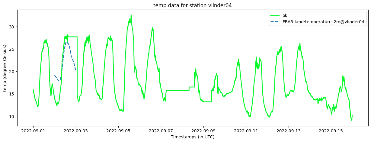
#Plot the modeldata and observational temperatures of a single station
dataset.get_station('vlinder04').make_plot(obstype='temp', show_modeldata=True)
[19]:
<Axes: title={'center': 'temp data for station vlinder04'}, xlabel='Timestamps (in UTC)', ylabel='temp (degree_Celsius)'>
[20]:
#Interactive spatial plot of the GEE dataset (with the stations as markers)

dataset.make_gee_plot(
    geedatasetmanager=era5_manager,
    timeinstance=pd.Timestamp('2022-09-02 13:00:00'),
    modelobstype='temp',
    vmax=None, #if None, the colorscale is optimalized for the extend of all stations
    vmin=None, #if None, the colorscale is optimalized for the extend of all stations
    )
[20]:
Transfer of larger amounts of data#
There is a limit to the amount of data that can be transferred directly from GEE. When the data cannot be transferred directly, it will be written to a file on your Google Drive. The location of the file will be printed out. When the writing to the file is done, you must download the file and import it using the Dataset.import_gee_data_from_file() method.
Note: The reason not to check the read-only option upon GEE authentication is to enable possibility to write files to your google drive.
As a demonstration we download the temperature and pressure timeseries from ERA5-land, for all the stations and for the same period as the observations (15 days). This amount of data is to large to transfer directly.
[21]:
#Extract the timeseries
_nothing_returned = dataset.get_gee_timeseries_data(
            geedynamicdatasetmanager=era5_manager, #The datasetmanager to use
            startdt_utc=None, #If None, the startdt of the dataset observations is used
            enddt_utc=None, #If None, the startdt of the dataset observations is used
            target_obstypes=['temp', 'pressure'], #the observationtypes to extract, must be knonw modelobstypes
            )
WARNING:<metobs_toolkit>:THE DATA AMOUNT IS TOO LARGE FOR INTERACTIVE SESSION, THE DATA WILL BE EXPORTED TO YOUR GOOGLE DRIVE!
WARNING:<metobs_toolkit>:The timeseries will be written to your Drive in gee_timeseries_data/ERA5-land_timeseries_data_of_full_dataset_28_stations
WARNING:<metobs_toolkit>:The data is transfered! Open the following link in your browser:


WARNING:<metobs_toolkit>:https://drive.google.com/#folders/1QE0DA-YqeHh5gSUG2L1EWh7ndyxa7xNj


WARNING:<metobs_toolkit>:To upload the data to the model, use the Dataset.import_gee_data_from_file() method.
WARNING:<metobs_toolkit>:No data is returned by the GEE api request.
The data request was to big for direct transfer, a (CSV) file is written to your Google Drive (See the link in the printed warning).
Download that file, and then import the modeldata from the file.
[22]:
%%script true

#Import the ERA5 data
dataset.import_gee_data_from_file(
        filepath= '... path to the downloaded file ...',
        geedynamicdatasetmanager=era5_manager
        )
Extending the defaults#
The default GeeDatasetManager are illustrative and they may not be sufficient. Here are some demonstrations on how to extend upon the defaults.
Using a new ModelObstype#
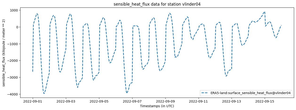
In this demo we add the surface sensible heat flux as a new modelobstype and download the timeseries at the location of the stations.
See the details of the ERA5-land dataset.
[23]:
#1. Create a observation type
sensible_heat_flux = metobs_toolkit.Obstype(
                        obsname='sensible_heat_flux',
                        std_unit='kJ/m^2',
                        description='The 2m sensible heat flux.')

#2. Make a ModelObstype
sensible_heat_flux_era5 = metobs_toolkit.ModelObstype(
                            obstype=sensible_heat_flux,
                            model_unit='J/m^2', #see details on GEE
                            model_band='surface_sensible_heat_flux') #see details on GEE

#3. Add the ModelObstype to the dataset manager
era5_manager = metobs_toolkit.default_GEE_datasets['ERA5-land']
era5_manager.add_modelobstype(sensible_heat_flux_era5)


#4. Extract some sensible heat flux data (for a single station as demo)
sens_heat_flx_data = dataset.get_station('vlinder04').get_gee_timeseries_data(
                        geedynamicdatasetmanager=era5_manager,
                        startdt_utc=None,
                        enddt_utc=None,
                        target_obstypes=['sensible_heat_flux'] #refer by obsname
                        )
#The sensible heat flux data is stored as modeldata in the station (if the direct transfer is succescfull!)

#5. make a plot
dataset.get_station('vlinder04').make_plot_of_modeldata(obstype='sensible_heat_flux')

#6. You can also get the data using the modeldatadf attribute
dataset.get_station('vlinder04').modeldatadf
[23]:
| value | details | ||
|---|---|---|---|
| datetime | obstype | ||
| 2022-09-01 00:00:00+00:00 | sensible_heat_flux | -2671.636963 | ERA5-land:surface_sensible_heat_flux converted... |
| 2022-09-01 01:00:00+00:00 | sensible_heat_flux | 156.804245 | ERA5-land:surface_sensible_heat_flux converted... |
| 2022-09-01 02:00:00+00:00 | sensible_heat_flux | 286.745514 | ERA5-land:surface_sensible_heat_flux converted... |
| 2022-09-01 03:00:00+00:00 | sensible_heat_flux | 417.542999 | ERA5-land:surface_sensible_heat_flux converted... |
| 2022-09-01 04:00:00+00:00 | sensible_heat_flux | 551.778992 | ERA5-land:surface_sensible_heat_flux converted... |
| ... | ... | ... | ... |
| 2022-09-15 20:00:00+00:00 | sensible_heat_flux | -287.355988 | ERA5-land:surface_sensible_heat_flux converted... |
| 2022-09-15 21:00:00+00:00 | sensible_heat_flux | -172.500000 | ERA5-land:surface_sensible_heat_flux converted... |
| 2022-09-15 22:00:00+00:00 | sensible_heat_flux | -58.152000 | ERA5-land:surface_sensible_heat_flux converted... |
| 2022-09-15 23:00:00+00:00 | sensible_heat_flux | 30.048000 | ERA5-land:surface_sensible_heat_flux converted... |
| 2022-09-16 00:00:00+00:00 | sensible_heat_flux | 99.676003 | ERA5-land:surface_sensible_heat_flux converted... |
386 rows × 2 columns
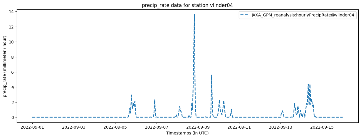
Defining a new GEE dataset#
In this example we create a new GeeDyanamicDatasetManager that is a JAXA reanalysis product for global precipitation, see JAXA_GPM_L3_GSMaP_v8_operational details.
[24]:
#1. Create an pricipitation observationtype

precip_rate = metobs_toolkit.Obstype(obsname='precip_rate',
                                     std_unit='mm/hour',
                                     description='Rain precipitation rate at surface.')
#2. Create a ModelObstype
precip_GPM = metobs_toolkit.ModelObstype(
                obstype=precip_rate,
                model_unit='mm/hour', #See GEE dataset details
                model_band='hourlyPrecipRate',#See GEE dataset details
                )

#3. Create a ModelDataManager
GPM_v8_manager = metobs_toolkit.GEEDynamicDatasetManager(
    name='JAXA_GPM_reanalysis',
    location="JAXA/GPM_L3/GSMaP/v8/operational", #See GEE dataset details
    value_type='numeric',
    scale=50,
    time_res='1h',
    modelobstypes=[precip_GPM],
    is_image=False,
    is_mosaic=False,
)

#4. Extract precipitation timeseries data
precip_data = dataset.get_station('vlinder04').get_gee_timeseries_data(
                        geedynamicdatasetmanager=GPM_v8_manager,
                        startdt_utc=None,
                        enddt_utc=None,
                        target_obstypes=['precip_rate'] #refer by obsname
                        )

# 5. make a plot
dataset.get_station('vlinder04').make_plot_of_modeldata(obstype='precip_rate')

# 6. You can also get the data using the modeldatadf attribute
dataset.get_station('vlinder04').modeldatadf
[24]:
| value | details | ||
|---|---|---|---|
| datetime | obstype | ||
| 2022-09-01 00:00:00+00:00 | precip_rate | 0.000000 | JAXA_GPM_reanalysis:hourlyPrecipRate converted... |
| sensible_heat_flux | -2671.636963 | ERA5-land:surface_sensible_heat_flux converted... | |
| 2022-09-01 01:00:00+00:00 | precip_rate | 0.000000 | JAXA_GPM_reanalysis:hourlyPrecipRate converted... |
| sensible_heat_flux | 156.804245 | ERA5-land:surface_sensible_heat_flux converted... | |
| 2022-09-01 02:00:00+00:00 | precip_rate | 0.000000 | JAXA_GPM_reanalysis:hourlyPrecipRate converted... |
| ... | ... | ... | ... |
| 2022-09-15 22:00:00+00:00 | sensible_heat_flux | -58.152000 | ERA5-land:surface_sensible_heat_flux converted... |
| 2022-09-15 23:00:00+00:00 | precip_rate | 0.000000 | JAXA_GPM_reanalysis:hourlyPrecipRate converted... |
| sensible_heat_flux | 30.048000 | ERA5-land:surface_sensible_heat_flux converted... | |
| 2022-09-16 00:00:00+00:00 | precip_rate | 0.000000 | JAXA_GPM_reanalysis:hourlyPrecipRate converted... |
| sensible_heat_flux | 99.676003 | ERA5-land:surface_sensible_heat_flux converted... |
747 rows × 2 columns
[25]:
#Or you can make an interactive spatial plot
dataset.make_gee_plot(
        geedatasetmanager=GPM_v8_manager,
        modelobstype='precip_rate',
        timeinstance=pd.Timestamp('2022-09-08 16:00:00'))
[25]: